WAREHOUSE BANKING

∗

Jason Roderick Donaldson Giorgia Piacentino Anjan Thakor

Washington University in St. Louis

August 31, 2015

Abstract

We develop a new theory of banking that provides a view of liquidity creation that

diﬀers signiﬁcantly from the existing paradigm. The theory links modern-day banks to

their historical origin as warehouses. When the warehouse accepts deposits, it issues

“warehouse receipts,” claims on deposits it safeguards, as “proof” of deposits, but this

suﬃces neither to create liquidity nor to make the warehouse a bank. Our main result is

that the warehouse becomes a bank and creates ex ante aggregate liquidity only when it

makes loans in “fake” receipts—i.e. receipts that are observationally identical to authen-

tic receipts, but are not backed by dep osits. In other words, what creates liquidity and

economic growth is not banks’ deposit-taking per se—banks issuing receipts in exchange

for the deposit of goods—but rather the combination of this with account-keeping (i.e.

warehousing) and fake-receipt-based lending. On the policy front our theory suggests

that the currently-contemplated suggestions to have narrow banking or impose liq-

uidity requirements will inhibit aggregate liquidity creation, whereas increasing bank

capital will enhance bank liquidity creation. This stands in contrast with the policy

prescriptions of models of bank liquidity creation based on deposit-taking and lending

but without warehousing and fake-receipt issuance. We also show that a tighter central

bank monetary policy does not always reduce liquidity creation—we provide conditions

under which it leads to higher liquidity creation by banks.

∗

For their helpful comments, we thank Franklin Allen, Ulf Axelson, Juliane Begena u, Liam Br unt, Mike

Burkart, Doug Dia mond, Co lm Friel, Anand Goel, Itay Goldstein, Charles Goodhart, Denis Gromb, Charles

Kahn, Peter Koudijs, Andrey Malenko, Nadya Malenko, Clemens Otto, George Pennacchi, Uday Rajan,

Adriano Rampini, Javier Suarez, Lucy White, Andrew Winton, Randy Wr ight and seminar par ticipa nts at

the Sixth Bank of Po rtugal Conference on Financial I ntermediation, the 2015 European Summer Symposium

in Financial Markets at Gerzensee, the 2015 IDC Summer Finance Conference, the 2015 Summer Money

Workshop at the St Louis Fed, and Washington University in St. Louis. We alone ar e responsible for any

remaining errors.

The banks in their lending business are not only not limited by their own

capital; they are not, at least immediately, limited by any capital whatever; by

concentrating in their hands almost all payments, they themselves create the

money required...

Wicks ell (1907)

Introduction

Banking is an old business. The invention of banking precedes the invention of coinage

by several thousand years.

Banks evolved from ancient warehouses, where cattle, grain,

and precious metals were depos ited for storage. For example, in ancient Egypt, grain

harvests were “deposited” (or stored) in centralized warehouses and depositors could

write orders for the withdrawal of certain quantities of grain as means of payment.

These orders constituted some of the earliest paper money. Eventually the warehouses

for the safe storage of commodities began making loans, thereby evolving into modern

banks (see Williams (1986) and Lawson (1855), for example). By extending credit, these

institutions transformed from simple warehouses of liquidity to creators of liquidity. To

this day, the same institutions that provide safekeeping services also engage in the

bulk of lending in the economy and are responsible for signiﬁcant liquidity creation

(e.g., Berger and Bouwman (2009)). Modern commercial and retail banks keep deposit

accounts, provide payment services and act as custodians as well as make corporate

and consumer loans.

Why do modern banks oﬀer deposit-taking, account-keeping, payment, and custodial—

namely, warehousing—services within the same institution that provides lending ser-

vices? How do banks that combine warehousing and lending services create liquidity?

What does a theory of banking that addresses these questions have to say about regu-

latory initiatives like bank capital and liquidity requirements and proposals like narrow

banking?

In this paper, we address these questions by developing a model of banking based

on the warehousing function of the bank. In our model, the institutions that provide

the warehousing services endogenously perform the lending in the economy. The model

relies on two key assumptions. First, warehouses have an eﬃcient storage technology

and, second, no ﬁrm’s output is pledgeable,

so debt written on a ﬁrm’s future cash

ﬂow is not readily enforceable. Warehouses use their superior storage technology to

Banking seems to have originated in ancient Mesopotamia and some of the earliest recorded laws per-

taining banks (banking reg ulation) were part of the Code of Hammurabi.

See Ho lmström and Tiro le (2 011) for a list of “...several reasons why this [non-pledgeability] is by and

large reality” (p. 3).

circumvent the non-pledgeability problem. The warehouse’s ability to do this stems

from the fact that it is costly for ﬁrms to store their output privately, so they want to

deposit their output in a warehouse that can store it at a lower cost.

However, once

a ﬁrm deposits with the warehouse, the deposit can then be seized by the warehouse.

Thus, when the costs to private storage are high enough, it becomes incentive compat-

ible for ﬁrms to repay their debts in order to access warehouses’ storage services. This

mechanism explains why the same institutions should provide both the warehousing

and lending services in the economy.

Our model of warehouse banking leads to a new perspective on banks’ liquidity

creation. In our model, as in ancient Egypt, the receipts that warehouses issue for

deposits circulate as a medium of exchange—they constitute private money. This is

the ﬁrst step in the bank’s creation of funding liquidity, which we deﬁne as the bank-

linked elevation of the initial liquidity that is allocated to productive inves tments.

The

second step in the liquidity creation process—and the key reason that banks increase

aggregate funding liquidity—is that they make loans in warehouse receipts rather than

in deposited goods. When banks make loans, they issue new receipts—“fake receipts”—

that are not backed by any deposits. Despite the lack of deposit-backing, these receipts

provide ﬁrms with working capital, allowing them to make more productive investments.

Note that banks create ex ante liquidity only when they make loans in fake receipts. If

the warehouse only takes deposits and issues receipts for them, it creates no liquidity

because it is simply exchanging one liquid as set for another—exchanging a liquid receipt

for a liquid deposit of real goods or central bank money.

Our warehousing view of banking provides some new insights into ﬁnancial regu-

latory policy. One proposal is narrow banking. We interpret a narrow bank as an

institution that can invest its deposits in only “safe” assets, namely in cash or mar-

ketable liquid securities such as sovereign bonds (see Pennacchi (2012)). The proposal

forces the separation of the warehousing and lending functions of banks. Our analysis

suggests that banks create liquidity only when they perform this dual function, imply-

ing that narrow banks create no liquidity. Less extreme proposals, such as the liquidity

(reserve) ratio in Basel III, demand that banks invest at least a speciﬁed fraction of

their assets in cash and marketable liquid securities. These too stiﬂe banks’ liquidity

The assumption is somewhat similar to the a ssumption in Allen and Gale (1998) that the storage tech-

nology availa ble to ba nk s is strictly more productive than the storag e technology available to consumers. As

we discuss later, this cost advantage for the warehouse may also stem from being in a privileged position of

power, like the a ncie nt warehouses from which banks evolved; these were linked to places of worship and/o r

the k ing’s tre asury.

In support of this mechanism, Skrastins (2015) uses a diﬀerences-in-diﬀere nce s research design to demon-

strate that agricultural lenders in Brazil extend more credit when they merge with grain silos, i.e. banks

lend more when they are also warehouses.

We use the term “funding liquidity” in the sense in which it is used by Brunnermeier and Pedersen

(2009).

creation in our set-up, since they prevent banks from issuing fake receipts to expand the

supply of liquidity. In an extension, we contrast the eﬀect of liquidity requirements with

the eﬀ ect of capital (equity) requirements, which can actually enhance banks’ ability

to create liquidity by reducing moral hazard problems between banks and depositors,

making warehousing relatively more eﬃcient. We also extend the model to include a

central bank and argue that a tighter monetary policy does not alway s lead to lower

liquidity creation. We establish conditions under which such a policy can actually

encourage lending by warehouse-banks.

Our model stands in contrast to the contemporary literature on why banks exist.

The only assumption we make on banks is that they have a storage technology. They

have no superior ability to screen or to monitor loans in an environment of asymmetric

information, as in Diamond (1984) and Ramakrishnan and Thakor (1984). Because we

assume that all agents are risk neutral, banks also do not provide better risk sharing for

risk averse depositors as in Bryant (1980) and Diamond and Dybvig (1983). Technolog-

ical and ﬁnancial developments have diminished informational frictions and provided

alternatives to banks for risk-sharing (see the discussion in Coval and Thakor (2005)).

This s hould have led to a decline in ﬁnancial intermediaries’ share of output (and cor-

porate proﬁts) in developed economies, but their ﬁnancial sectors have continued to

grow. This suggests that other forces also determine the demand for banking services;

we suggest that warehousing-type ﬁnancial services may be one important determinant,

one linked with the very origins of banking. In fact, the largest deposit bank in the

world today, Bank of New York–Mellon, is usually classiﬁed as a custodian bank, i.e.

an institution responsible for the safeguarding, or warehousing, of ﬁnancial assets.

Our paper is also related to the literature on liquidity creation by banks which relies

on the role of intermediaries as providers of liquidity insurance. Important contribu-

tions include Allen and Gale (1998), Allen, Carletti, and Gale (2014), Bryant (1980),

Diamond and Dybvig (1983), and Postlewaite and Vives (1987). In our model, banks

create liquid securities, since they issue receipts that constitute private money, and they

also create aggregate liquidity since more capital is directed into productive investment

with the bank than without. In other words, banks enhance funding liquidity. This

contrasts with the model in Diamond and Dybvig (1983) and other models of that genre

in at least ﬁve important respects, discussed below.

First, in Diamond and Dybvig (1983), the bank creates liquid securities, namely

demand-deposit contracts, to raise funds to invest in illiquid projects. However, the

bank does not create aggregate funding liquidity, since no more is invested in the illiq-

uid projects than would be absent the bank. In our model, the bank creates aggregate

funding liquidity precisely because it can create liquid securities—warehouse receipts—

with which to make loans. Since the receipts circulate as a medium of exchange, they

provide working capital to ﬁrms, expanding the total supply of liquidity available for

investment. Second, in existing models of bank liquidity creation, aggregate investment

is typically bounded by the total initial endowment of liqui dity in the economy. Banks

are limited to taking deposits and lending them out. Not so in our model. Indeed, in

aggregate ﬁrms invest in more capital and labor than the initial aggregate endowment of

liquidity in the economy, something that is impossible with the non-bank direct invest-

ment outcome. That is, in our model, lending also creates deposits. Third, models like

Bryant (1980) and Diamond and Dybvig (1983) focus on the bank’s interactions with

depositors as the source of liquidity creation, with uncertainty about time preferences

creating a preference for liquidity by (risk-averse) dep ositors. In other words, liquidity

creation is viewed as being synonymous with consumption insurance—the bank pro-

vides risk averse depositors with higher interim consumption than possible with direct

investment in the project that the bank invests its deposits in. Thus, even though the

depositor has just as liquid an asset by keeping his money in his pocket as he does by

depositing it in a bank, he obtains higher interim consumption and hence better risk

sharing with a deposit.

In contrast, our model focuses on the asset side of the bank’s

balance s heet as a result of our diﬀerent deﬁnition of liquidity creation. Fourth, in the

existing models of bank liquidity creation, coordination failures among depositors can

lead to bank runs, an issue that does not arise in our model. Finally, while in the

existing models bank capital either plays no role in liquidity creation or is viewed as

impeding bank liquidity creation, in our model we show that it enhances bank liquidity

creation.

This focus on the bank’s assets, along with our assumption that all agents are

risk neutral, means that bank liquidity creation is decoupled from risk preferences.

Risk sharing for depositors is thus neither necessary nor suﬃcient for ex ante liquidity

creation by the bank in our framework, although deposits are an important reason why

the bank exists in the ﬁrst place. Liquidity creation is manifested through the lending

of fake receipts. In this sense, our approach in which bank lending creates deposits is

reminiscent of Hahn (1920):

We thus maintain—contrary to the entire literature on banking and credit—

that the primary business of banks is not the liability business, especially

the deposit business, but in general and in each and every case an asset

transaction of a bank must have previously taken place, in order to allow

the possibility of a liability business and to cause it. The liability business

of banks is nothing but a reﬂex of prior credit extension.... (H ahn, 1920, p.

29)

Jacklin (1987) shows that if the owner of the project that the bank invests in were to issue traded equity

that paid a dividend at the interim date, the same risk sharing can be achieved as provided by bank deposits.

See also Werner (2014) and the “g oldsmith anecdote” in Greenbaum, Thakor, and Boot (2015)

Keynes makes a related point:

It is not unnatural to think of deposits of a bank as being created by the

public through the deposits of cash representing either savings or amounts

which are not for the time being required to meet expenditures. But the

bulk of the deposits arise out of the action of the banks themselves, for by

granting loans, allowing money to be drawn on an overdraft or purchasing

securities, a bank creates a credit in its books which is the equivalent of a

deposit. (Keynes in his contribution to the Macmillan Committee, 1931, p.

34)

We view our paper as oﬀering a view of bank liquidity creation that complements the

consumption insurance view in the existing literature, a view that has provided deep in-

sights into a variety of phenomena like bank runs and deposit insurance (Bryant (1980)

and Diamond and Dybvig (1983)), ﬁnancial crises (e.g. Allen and Gale (1998)), and the

role of ﬁnancial intermediaries vis-à-vis markets (e.g. Allen and Gale (2004)). Juxta-

posing our analysis with the existing literature, liquidity creation is seen to have two

important dimensions: consumption insurance for depositors/savers and elevated fund-

ing liquidity for entrepreneurs/borrowers. These mutually-reinforcing views of bank

liquidity creation are consistent with the idea that banks create liquidity by both tak-

ing in deposits and selling loan commitments (e.g. Kashyap, Rajan, and Stein (2002)).

In addition to providing a diﬀerent perspective on the role of banks and what they

do to create liquidity, our paper also provides a microfoundation for the assumption

that cash ﬂow diversion destroys value, which is common in the ﬁnance literate (e.g.

Bolton and Scharfstein (1990) and Hart and M oore (1998)). In these models, if a bor-

rower diverts his cash ﬂow rather than repays his creditor, his cash ﬂow typically de-

creases by an exogenous, borrower-speciﬁc constant. In our model, such a number arises

endogenously as the ratio of depreciation given private storage to the returns on the

warehouses’ technology. Note that this suggests that the costs of diversion should not

be borrower-speciﬁc in general, in the sense that they depend not only on the borrower’s

technology, but on the creditor’s technology as well.

The rest of the paper is organized as follows. Section 2 provides an example in a

simpliﬁed set-up in which all the key forces of the model are at work. Section 3 develops

the formal model. Section 4 contains the solution of the model. Section 5 s olves two

benchmark models: (i) one in which warehouses cannot issue fake receipts and (ii) the

ﬁrst-best allocation. Section 6 contains the main results. It presents analysis of liquidity

creation and fractional reserves. Section 7 considers the welfare implications of four

policies: liquidity requirements, narrow banking, capital requirements, and monetary

policy. Finally, Section 8 concludes. The appendix contains all proofs and a glossary

of notation.

2 Motivating Example

In this subsection, we write a numerical example that illustrates the main mechanism at

work in a simpliﬁed setup. We write the example with just three players, one farmer,

one laborer, and one warehouse. We examine a sequence of increasingly rich cases

to demonstrate the eﬃciency gains from warehousing and from issuing fake receipts.

Speciﬁcally, we consider: (1) the case without a warehouse, (2) the case in which a

warehouse provides only safe-keeping services but does not lend, (3) the case in which a

warehouse provides both safe-keeping and lending services, and (4) the ﬁrst-best case,

in which the allocation is eﬃcient.

The analysis of the example shows that, even without lending, warehousing alone

increases eﬃciency by providing more eﬃcient storage. This eﬃciency gain is merely

technological, however; introducing a better storage technology increases terminal out-

put. But when a warehouse can issue f ake receipts, it does more to improve eﬃciency.

By issuing fake receipts, the warehouse creates liq uidity th at the farmer invests produc-

tively. This eﬃciency gain is allocational and is much more important than the simple

technological eﬃciency gain. When the warehouse issues fake receipts, it allows other

players in the economy to invest in more eﬃcient technologies. Finally, the analysis

of the ﬁrst-best allocation suggests that there is an eﬃciency loss in the second bes t

even when the warehouse can is sue fake receipts, it still creates less liquidity than in

the ﬁrst-best.

The setup of the example is as follows. There are three dates, Date 0, Date 1, and

Date 2. The farmer has an endowment e of twelve units of grain at Date 0 and no one

else has any grain. At Date 0 the farmer can borrow B from the warehouse at gross

rate one. We assume that warehouse dep os it rates and wages w are also all set equal

to one.

The farmer produces over the period from Date 0 to Date 1 and he stores his

output over the period from Date 1 to Date 2. I f the farmer stores his grain privately, it

depreciates at δ percent, and we choose to set δ = 20%; if he stores it in a warehouse, it

does not depreciate. This can be viewed as the warehouse havi ng better defense against

theft, for reasons we explain later. The farmer’s production technology transforms a

unit of labor and a unit of grain at Date 0 into f our units of grain at Date 1 with

constant returns. In other words, the farmer has a Leontief p roduction function in the

ﬁrst perio d that takes grain investment i, which we will refer to as “capital investment,”

and labor ℓ and produces output y = 4 min {i, ℓ} at Date 1. We assume that this output

is not pledgeable; however, a warehouse can seize the deposits it holds. Suppose there

is no discounting, so workers are willing to store grain in warehouses at the deposit rate

These prices—i.e. rates and wages—result from competition in the full model, leaving rents to the farmer.

We ta ke them as given in this example for simplicity.

of one. Everyone consumes only at Date 2.

The parameter values are summarized in Figure 1 and the timing is illustrated in

Figure 2.

Figure 1: Summary of notation and values in example in Section 2 .

Quantity

Notation Value in Example

Farmer’s endowment e 12

Farmer’s technology

y 4 min {i, ℓ}

Depreciation rate δ 20%

Wage

w 1

Figure 2: A Simplified Timeline Representation of the Sequence of Moves

Date 0

the farmer has endowment e and borrows B from the warehouse

he invests i in grain, and wℓ in labor

the lab orer exerts la bor ℓ and deposits his wages wℓ in the warehouse

Date 1

the farmer produces y

he either repays and deposits or diverts and stores privately

Date 2

the farmer, laborer, and warehouse consume

Deﬁnition of liquidity creation: We refer to the farmer’s expenditure on capital

and labor i + wℓ as the “total investment.” We measure liquidity creation by the ratio

Λ of the farmer’s total investment to his initial endowment,

Λ =

i + wℓ

No warehousing. Consider ﬁrst the case in which there is no warehousing. Thus,

the farmer must pay the laborer in grain. To maximize his Date 2 consumption, the

farmer maximizes his Date 1 output and then stores his output from Date 1 to Date

2. To maximize his Date 1 output, he invests in equal amounts of capital i and labor ℓ

(as a result of the Leontief technology). Since his endowment is twelve and wages are

one, he sets i = ℓ = 6 and produces y = 4 × 6 = 24 units of grain. He then stores his

grain privately from Date 1 to Date 2 and this grain depreciates by twenty percent; the

farmer’s ﬁnal payoﬀ is (1 − 20%) × 24 = 19.2 units. Λ

= 1, so there is no liquidity

creation.

Warehousing but no fake receipts. Now consider the case where there is a

warehouse, but that it performs only the function of safekeeping. When a depositor

(the farmer or the laborer) deposits grain in the warehouse, the warehouse issues receipts

and holds the grain until it is withdrawn. In this case, the farmer again maximizes his

Date 1 output in order to maximize his Date 2 consumption. Again, he will invest

equal amounts of capital and labor. He cannot borrow from the warehouse, so he again

just divides his endowment ﬁfty-ﬁfty between capital investment and labor, setting

i = ℓ = 6 and producing y = 4 × 6 = 24 units of grain. He now s tores his grain in the

warehouse from Date 1 to Date 2. Since it is warehoused, the grain does not depreciate;

the farmer’s ﬁnal payoﬀ is 24 units. Warehousing has added 4.8 units to the farmer’s

consumption by increasing eﬃciency in storage. But the warehouse has not created any

liquidity for the farmer since the initial investment in the technology i + wℓ = e = 12 is

the same as in the case in which there is no warehouse. There is no liquidity creation,

= 1.

Warehousing with fake receipts. Now consider the case in which there is a

warehouse that provides not only safe-keeping but also lends. Since the farmer’s tech-

nology is highly productive, he wishes to borrow to scale it up. But the farmer already

holds all twelve units of grain in the economy, so how can he scale up his production

even further? The key is that the f armer can borrow from the warehouse in warehouse

receipts. Observe that the receipts the warehouse uses to make loans are n ot backed

by grain; they are “fake receipts.” However, if the laborer accepts payment from the

farmer in these fake receipts, they are still valuable to the farmer—they provide him

with “working capital” to pay the laborer.

The farmer again s ets his capital investment equal to his labor investment, i = ℓ.

Given that he can borrow B in receipts from the warehouse, however, he can now

invest a total up to i + wℓ = e + B. Thus, recalling that wages w are one, his optimal

investment is

i =

e + B

= 6 +

(1)

and the corresponding Date 1 output is

y = 4i = 24 + 2B. (2)

Given that this technology is highly productive and has constant returns to scale, the

farmer wishes to expand production as much as possible. The amount he can borrow

from the warehouse, however, is limited by the amount that he can credibly promise to

repay. Since we have assumed that the farmer’s output is not pledgeable, his creditor

(i.e., the warehouse) cannot enforce the repayment of his debt. However, if the farmer

deposits in the warehouse, it is possible for the warehouse to seize the deposit. Thus,

after the farmer produces, he faces a tradeoﬀ between not depositing and depositing.

If he does not deposit, he stores privately, so his grain depreciates, but he avoids

repayment. If he does dep osit, he avoids depreciation, but the warehouse can seize his

deposit and force repayment. The warehouse lends to the farmer only if repayment is

incentive compatible. For the repayment to be incentive compatible, the farmer must

prefer to deposit in the warehouse and repay his debt rather than to store the grain

privately and default on his debt. This is the case if the following inequality holds

y − B ≥ (1 − 20%)y. (3)

The maximum the farmer can borrow B is thus given by



24 + 2B



− B =



1 − 20%



24 + 2B



, (4)

or B = 8. This corresponds to i = ℓ = 10. The liquidity creation is given by

Λ =

i + wℓ

10 + 10

. (5)

The farmer is able to scale up his production only when the warehouse makes

loans by writing fake receipts. In other words, liquidity is created on the asset side,

not the deposit side, of the warehouse’s balance sheet. When a warehouse makes a

loan, it creates both an illiquid asset, the loan, and a liquid liability, the fake receipt.

This is liquidity transformation, one of the fundamental economic roles of banks. Our

model suggests, however, that liquidity transformation occurs entirely when banks make

loans—it is not necessary that banks fund themselves with liquid deposits and then,

separately, make illiquid loans.

If the farmer could pay the labor on credit, he would not need to borrow from the

warehouse and he could expand production even further. However, an impediment to

this is that the laborer cannot enforce repayment from the farmer (because the output is

not pledgeable and the laborer has no way to seize it). Therefore, the farmer’s promise

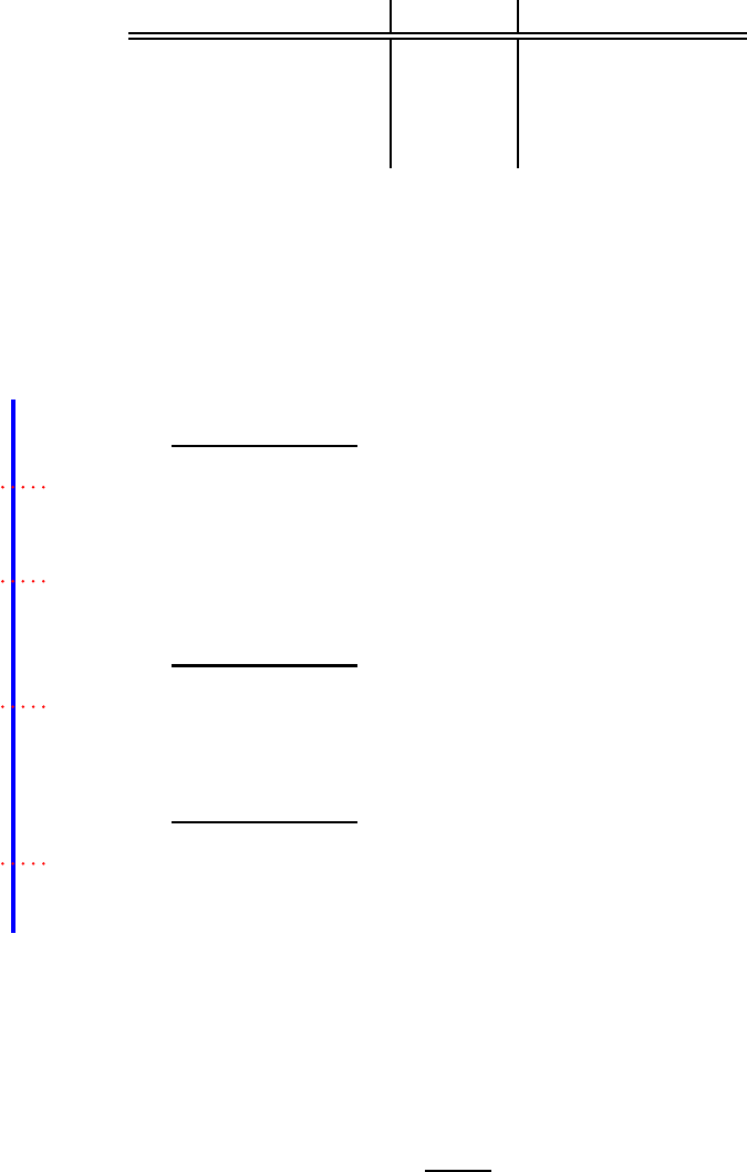
Figure 3: The warehouse’s balance sheet expands when it makes a loan, cre-

ating liquidity.

Balance sheet before lending Balance sheet after lending

grain receipts grain receipts

liquidity creation

−−−−−−−−−−−−→

loan fake receipts

to the laborer is not credible.

First-best. We now consider the ﬁrst best allocation of resources in order to

emphasize that the incentive compatibility constraint limits liq uidity creation. Allowing

warehouses to make loans in fake receipts moves the economy closer to the ﬁrst best

level of liquidity creation, but does not achieve it. In the ﬁrst-best allocation the farmer

invests his entire endowment in capital i = e = 12 and laborers exert equal labor ℓ = 12.

In this allocation output y = 4i = 48 and liquidity creation is given by

i + wℓ

12 + 12

= 2. (6)

Figure 4: Summary of liquidity creation the example in Section 2.

Case

Date 1 Output y Date 2 Output Liquidity Λ

No warehouses 24 19.2 1

Warehouses without lending 24 24 1

Warehouses with lending

40 40 5/3

First-best 48 48 2

Model

There are three dates, Date 0, Date 1, and Date 2 and three groups of players, farmers,

warehouses, and laborers. There is a unit continuum of each type of player. There

is one real good, called grain, which serves as the numeraire. There are also receipts

issued by warehouses, which entail the right to withdraw grain from a warehouse.

All players are risk neutral and consume only at Date 2. Denote farmers’ consump-

tion by c

, laborers’ consumption by c

, and the warehouses’ consumption by c

(the

index b stands for “bank”). Farmers begin life with an endowment e of grain. No other

player has a grain endowment. Laborers have labor at Date 0. They can provide labor

ℓ at the constant marginal cost of one. So their utility is c

− ℓ. Farmers have access

to the following technology. At Date 0, a farmer invests i units of grain and ℓ units of

labor. At Date 1, this investment yields

y = A min {αi, ℓ} , (7)

i.e. the production function is Leontief. The output y is not pledgeable. At Date 1

farmers have no special production technology: they can either store grain privately or

store it in a warehouse.

If grain is not invested in the technology, it is either stored privately or stored in a

warehouse. If the grain is stored privately (by either farmers or laborers), it depreciates

at rate δ ∈ [0, 1). If player j stores s

units of grain privately from Date t to Date t + 1,

he has (1 − δ)s

units of grain at Date t + 1. If grain is stored in a warehouse, it does

not depreciate. Further, if grain is stored in the warehouse, the warehouse can seize it.

The assumption that the warehouse can store grain more eﬃciently than the in-

dividual farmer has a natural interpretation in the context of the original warehouses

from which banks evolved. These ancient warehouses tended to be (protected) temples

or the treasures of sovereigns, so they had more power than ordinary individuals and a

natural advantage in safeguarding valuables and enforcing contracts.

Our assumption

on δ can thus be viewed either as a technological advantage arising from specializa-

tion acquired through (previous) investment and experience or as a consequence of the

power associated with the warehouse.

When players store grain in warehouses, warehouses issues receipts as “proof” of

these deposits. The bearers of receipts can trade them among themselves. Warehouses

can also issue receipts that are not proof of deposits. These receipts, which we refer to

as “fake receipts,” still entail the right to withdraw grain from a warehouse, and thus

they are warehouses’ liabilities that are not backed by the grain they hold. Receipts

We thank Charles Goodhart for this interpretation. Thus, whereas our focus is on private money (fake

receipts), the alternative, sovereign-power-linked interpretation of the storage advantage of the warehouse

over individuals means tha t our model may complement the chartalist view of money creation by the state

(e.g. Knapp (1924) and Minsky (2008)).

This power was important for several reasons that complement our approach and provide alternative

interpretations of the deep parameters in the model. First, it enabled grain, gold, or other valuable com-

modities to be s tored safely, without fear of robbery. Second, power enabled the creditor to impose greater

penalties on defaulting borrowers. Third, power also generated a greater likelihood of continuation of the

warehouse, and hence of engaging in a r e peated game with depositors. This created reputational incentives

for the warehouse not to abscond with deposits.

backed by grain are indistinguishable from fake receipts.

The markets for labor, warehouse deposits, and loans are competitive.

3.1 Financial Contracts

There are three types of contracts in the economy: labor contracts, deposit contracts,

and lending contracts. We restrict attention to bilateral contracts, although warehouse

receipts are tradeable and loans are also tradeable in an interbank market.

Lab or contracts are between farmers and laborers. Farmers pay laborers wℓ in

exchange for laborers’ investing ℓ in their technology, which then produces y = y(i, ℓ)

units of grain at Date 1.

Deposit contracts are between warehouses and the other players, i.e., laborers, farm-

ers, and (potentially) other warehouses. Warehouses accept grain deposits with gross

rate R

over one period, i.e. if player j ∈ {l, f } makes a deposit of d

units of grain

at Date t he has the right to withdraw R

units of grain at Date t + 1. When a

warehouse accepts a deposit of one unit of grain, it issues a receipt in exchange as

“proof” of the deposit.

Lending contracts are between warehouses and farmers. Warehouses lend L to

farmers at Date 0 in exchange for farmers’ promise to repay R

L at Date 1, where R

is the lending rate. Warehouses can lend in grain or in receipts. A loan made in receipts

is tantamount to a warehouse oﬀering a farmer a deposit at Date 0 in exchange for the

farmer’s promise to repay grain at Date 1. W hen a warehouse makes a loan in receipts,

we say that it is “issuing fake receipts.” We refer to a warehouse’s total deposits at

Date t as D

. These deposits include both those deposits backed by grain and those

granted as fake receipts.

Lending contracts are subject to a form of limited commitment on the farmers’ side.

Because farmers’ Date 1 output is not pledgeable, they are free to divert their output.

However, if the farmers do divert, they must store their grain privately. The reason is

that if they deposit their output in a warehouse, it may be seized by the warehouse.

We now formalize how we capture farmers’ inability to divert output if they deposit

in warehouses. We deﬁne the variable T as the total transfer from farmers to warehouses

at Date 1; T includes both the repayment of farmers’ debt to warehouses and farmers’

new deposits d

in warehouses. If farmers have borrowed B at Date 0, then they have

to repay R

B to warehouses at Date 1. W hen they make a transfer T to a warehouse at

Date 1, the “ﬁrst” R

B units of grain they transfer to the warehouse are used to repay

the debt. Only after full repayment of R

B do warehouses store grain for farmers as

deposits. Thus, the farmers’ deposits at Date 1 are given by

= T − min



T, R



= max



T − R

B, 0



. (DC)

This says that if farmers have not repaid their debt at Date 1, their Date 1 deposits

are constrained to be zero; we call this the deposit constraint.

The argument above glosses over one important subtlety. The farmer could borrow

from one warehouse at Date 0 and divert his output at Date 1, on ly to deposit his grain

in a diﬀerent warehouse. Would this allow the farmer to avoid both repaying his debt

and allowing his grain to depreciate? The answer is no. The reas on is as follows. If the

farmer deposits his grain in a warehouse that is not his original creditor, that warehouse

will buy the farmer’s debt from his original creditor on the interbank market, allowing

him to seize the grain the farmer owes. Thus, no matter which warehouse the farmer

deposits with, he will end up repaying his debt. We model the interbank market and

discuss this reasoning more formally in Appendix A.2.

Since there is no uncertainty, without loss of generality we can restrict attention to

lending contracts where default at Date 1 never happens in equilibrium. The farmer

will never default on his debt as long as repayment is incentive compatible. In other

words, he must prefer to repay his debt and deposit in the warehouse rather than to

default on his debt and store the grain privately. If g

denotes the farmer’s total Date

1 grain holding and R

B denotes the face value of his debt, then he repays his debt if

the following inequality is satisﬁed



− R



≥ (1 − δ)g

. (IC)

The timeline of moves for each player and their contractual relationships are illus-

trated in a timeline in Figure 5.

In equilibrium, the fa rmer’s total Date 1 grain holding g

comprises his Date 1 output y, his Date 0

deposits gross of interest, R

, and his depreciated savings (1 − δ)s

, or g

= y



i, ℓ



+ R

+ (1 − δ)s

Figure 5: A Timeline Representation of Sequence of Moves

Date 0

Warehouses

accept deposits D

lend L to farmers

store s

Farmers

borrow B from warehouses

invest i and ℓ in technology y

pay laborers wℓ

deposit d

in warehouses

store s

Laborers

exert labor ℓ

accept wage wℓ

deposit d

in warehouses

store s

Date 1

Warehouses

receive T from farmers

accept deposits D

repay R

to depositors

store s

Farmers

receive cash ﬂow y(i, ℓ)

transfer T to warehouses

receive R

from warehouses

have total grain holding g

deposit d

in warehouses

store s

Laborers

receive R

from warehouses

deposit d

in warehouses

store s

Date 2

Warehouses

repay R

to depositors

consume c

= s

− R

Farmers

receive R

from warehouses

consume c

= R

+ (1 − δ)s

Laborers

receive R

from warehouses

consume c

= R

+ (1 − δ)s

3.2 Summary of Key Assumptions

In this subsection, we restate and brieﬂy discuss the major assumptions underlying the

results.

Assumption 1. Output is not pledgeable.

This assumption prevents farmers’ from paying laborers directly in equity or debt. I f

farmers’ output were pledgeable, they could pay lab orers after their projects paid oﬀ.

Without this assumption, there would be no frictions and we could achieve the ﬁrst-best

allocation. Thus, this assumption creates a role for banks as providers of liquidity.

Assumption 2. Warehouses can seize the deposits they hold.

This as sumption implies that a warehouse can enforce repayment from a farmer as long

as that farmer chooses to deposit in it. Whenever farmers deposit in a warehouse, the

warehouse has a seizure technology that allows it to demand repayment from farmers.

This is one key ingredient to understand the connection between warehousing/account-

keeping and lending. As discussed above and in Appendix A.2, the interbank market

for loans prevents farmers from avoiding repayment by depositing in warehouses that

are not their creditors.

Assumption 3. Grain depreciates relatively more slowly if stored in a warehouse.

Speciﬁcally, we us e the normalization that grain does not depreciate inside a warehouse

and depreciates at rate δ ∈ (0, 1] outside a warehouse. This assumption gives farmers

a reason to deposit in warehouses rather than store grain themselves—farmers deposit

in warehouses to take advantage of more eﬃcient storage. This, in turn, ensures that

farmers will repay their debt, since warehouses can seize grain owed to them if it

is deposited with them, by Assumption 2. Thus, Ass umption 2 and As sumption 3

together imply that warehouses have a superior technology to enforce repay ment.

In some other theories of banking, the agents with the power to enforce contracts (or

“monitor borrowers”) naturally perform banking activities (e.g., Holmstrom and Tirole

(1997)). In our model, warehouse-banks’ enforcement power is an endogenous conse-

quence of their warehousing technology. Note that warehousing eﬃciency and enforce-

ment power are natural complements, as a superior warehousing technology may result

from the power to store assets safely, without f ear of robbery, as ex plained earlier.

Further, Assumption 2 implies that if a borrowers defaults, his access to warehousing

is limited in the future; this is analogous to warehouses’ having the power to impose

penalties on defaulting borrowers in a dynamic setting.

3.3 Individual Maximization Problems

All players take prices as given and maximize their Date 2 consumption subject to their

budget constraints. Farmers’ maximization problems are also subject to their incentive

compatibility constraint (IC).

We now write down each player’s maximization problem.

The warehouses’ maximization problem is

maximize c

= s

− R

(8)

over s

, s

, D

, and L subject to

= R

L + s

− R

+ D

, (BC

)

+ L = D

, (BC

)

and the non-negativity constraints D

≥ 0, s

≥ 0, L ≥ 0. To understand this maxi-

mization program, note that equation (8) says that the warehouse maximizes its proﬁt

(consumption) c

, which consists of the diﬀerence between what is stored in th e ware-

house at Date 1, s

, and what is paid to depositors, R

. Equation (BC

) is the

warehouse’s budget constraint at Date 1, which says that what is stored in the ware-

house at Date 1, s

, is given by the sum of the interest on the loan to the farmer, R

the warehouse’s savings at Date 0, the deposits at Date 1 D

minus the interest the

warehouse must pay on its time 0 deposits, R

. Similarly, Equation (BC

) is the

warehouse’s budget constraint at Date 0, which says that the sum of the warehouse’s

savings at Date 0, s

, and its loans L must equal the sum of the Date 0 deposits, D

The farmers’ maximization problem is

maximize c

= R

+ (1 − δ)s

(9)

over s

, s

, d

, T, i, ℓ

, and B subject to

= max



T − R

B, 0



, (DC)



− 1 + δ







i, ℓ



+ R

+ (1 − δ)s



≥ R

B, (IC)

T + s

= y



i, ℓ



+ R

+ (1 − δ)s

, (BC

)

+ s

+ i + wℓ

= e + B, (BC

)

and the non-negativity constraints s

≥ 0, d

≥ 0, B ≥ 0, i ≥ 0, ℓ

≥ 0, T ≥ 0. The

farmer’s maximization program can be understood as follows. In equation (9) the farmer

maximizes his Date 2 consumption c

, which consists of his Date 1 dep os its gross of

interest, R

, and his depreciated private savings, (1 − δ)s

. Equations (DC) and

(IC) are, respectively, the deposit constraint and the incentive compatibility constraint

(for an explanation see Subsection 3.1). The incentive compatibility constraint follows

directly from equation (IC) in Subsection 3.1, since the far mer’s Date 1 grain holding

comprises his Date 1 output y, his Date 0 deposits gross of interest, R

, and his

depreciated savings (1 − δ)s

, or g

= y



i, ℓ



+ R

+ (1 − δ)s

. Equation (BC

)

is the farmer’s budget constraint that says that the sum of his Date 1 savings, s

, and

his overall transfer to the warehouse, T , must equal the sum of his output y, his Date

0 deposits gross of interest, R

, and his depreciated savings, (1 − δ)s

. Equation

(BC

) is the farmer’s budget constraint at Date 0 which says that the sum of his Date

0 deposits, d

, his Date 0 savings, s

, his investment in grain i and his investment in

labor, wℓ

, must equal the sum of his initial endowment, e, and the amount he borrows,

The laborers’ maximization problem is

maximize c

= R

+ (1 − δ)s

− ℓ

(10)

over s

, s

, d

, and ℓ

subject to

+ s

= R

+ (1 − δ)s

, (BC

)

+ s

= wℓ

, (BC

)

and the non-negativity constraints s

≥ 0, d

≥ 0, ℓ

≥ 0. The laborer’s maximization

program can be understood as follows. In equation (10) the laborer maximizes his

Date 2 consumption c

, which consists of his Date 1 deposits gross of interest, R

and his depreciated private savings, (1 − δ)s

. Equation (BC

) is the laborer’s budget

constraint that says that the sum of his Date 1 savings, s

, and his Date 1 deposits, d

must equal the sum of his Date 0 deposits gross of interest, R

, and his depreciated

savings, (1 − δ)s

. Equation (BC

) is the laborer’s budget constraint at Date 0 which

says that the sum of his Date 0 deposits, d

, and his Date 0 s avings, s

, must equal his

labor income wℓ

3.4 Equilibrium

The equilibrium is a proﬁle of prices hR

, R

, wi for t ∈ {1, 2} and a proﬁle of alloca-

tions hs

, d

, D

, L, B, ℓ

, ℓ

i for t ∈ {1, 2} and j ∈ {b, f, l} that solves the warehouses’

problem, the farmers’ problem, and the laborers’ problem deﬁned in Section 3.3 and

satisﬁes the market clearing conditions for the labor market, the lending market, the

grain market and deposit market at each date:

ℓ

= ℓ

(MC

ℓ

)

B = L (MC

)

i + s

+ s

= e (MC

)

+ s

= (1 − δ)s

+ (1 − δ)s

+ s

+ y (MC

)

= d

+ d

(MC

)

= d

+ d

. (MC

)

3.5 Parameter Restrictions

In this section we make two restrictions on parameters. The ﬁrst ensures that farmers’

production technology generates suﬃciently high output that the investment is positive

NPV in equilibrium and the second ensures that the incentive problem that results

from the non-pledgeablity of farmers’ output is suﬃciently severe to generate a binding

borrowing constraint in equilibrium. Note that since the model is linear, if the farmers’

IC does not bind, they will scale their production inﬁnitely.

Parameter Restriction 1. The farmers’ technology is suﬃciently productive,

A > 1 +

. (11)

Parameter Restriction 2. Depreciation from private storage is not too fast,

δA < 1. (12)

Model Solution

In this subsection, we solve the model to characterize the equilibrium. We proceed

as follows. First, we pin down the equilibrium deposit rates, lending rates and wages.

Then we show that the model collapses to the farmer’s problem which we then s olve to

characterize the equilibrium.

4.1 Preliminary Results

Here we state three results that completely characterize all the prices in the model,

namely the two depos it rates R

and R

, the lending rate R

, and the wage w. We

then show that given the eq uilibrium prices, farmers and laborers will never store grain

privately. The results all follow from the deﬁnition of competitive equilibrium with

risk-neutral agents.

The ﬁrst two results say that the risk-free rate in the economy is one. This is natural,

since the warehouses have a scalable storage technology with return one.

Lemma 1. Deposit rates are one at each date, R

= R

= 1.

Now we turn to the lending rate. Since the farmers’ incentive compatibility con-

straint ensures that loans are riskless and warehouses are competitive, warehouses also

lend to f armers at rate one.

Lemma 2. Lending rates are one, R

= 1.

Finally, since laborers have a constant marginal cost of labor, the equilibrium wage

must be equal to this cost; this says that w = 1, as summarized in Lemma 3 below.

Lemma 3. Wages are one, w = 1.

Note that we have omitted the eﬀect of discounting in the pr e ceding argument—laborers work at Date

0 and consume at Date 2; discounting is safely forgotten, though, since the laborers have access to a riskless

storage technology with r e tur n one via the warehouses, as esta blished above.

These results establish that the risk-free rate oﬀered by warehouses exceeds the rate

of return from private storage, or R

= R

= 1 > 1−δ. Thus, farmers and laborers do

not wish to make use of their private storage technologies. The only time a player may

choose to store grain outside a warehouse is if a farmer diverts his output; however,

the farmer’s incentive compatibility constraint ensures he will not do this. Corollary 1

below summarizes this reasoning.

Corollary 1. Farmers and laborers do not store grai n, s

= s

= 0.

4.2 Equilibrium Characterization

In this section we characterize the equilibrium of the model. We proceed as follows.

First, we show that given the equilibrium prices established in Subsection 4.1 above,

laborers and warehouses are indiﬀerent among all allocations. We then establish that a

solution to the farmers’ maximization problem given the equilibrium prices is a solution

to the model.

The prices R

, R

, and w are determined exactly so that the markets clear

given that agents are risk-neutral. In other words, they are the unique prices that

prevent the demands of warehouses or laborers from being inﬁnite. This is the case

only if warehouses are indiﬀerent between demanding and supplying deposits and loans

at rates R

, R

, and R

and laborers are indiﬀerent between supplying or not supplying

labor at wage w. This implies that all prices are one in equilibrium, as summarized in

Lemma 4 below.

Lemma 4. Given the equilibrium prices, R

= R

= w = 1, warehouse are

indiﬀerent among all deposit and loan amounts and laborers are indiﬀerent among all

labor amounts.

Lemma 4 implies that, given the equilibrium prices, they will absorb any excess

demand left by the farmers. In other words, given the equilibrium prices established in

Subsection 4.1 above, for any solution to the farmer’s individual maximization problem,

laborers’ and warehouses’ demands are such that markets clear.

We have thus established that the equilibrium allocation is given by the solution

to the farmers’ problem given the eq uilibrium prices, where the laborers’ and ware-

houses’ demands are determined by the market clearing conditions. Thus, to ﬁnd the

equilibrium, we maximize the farmers’ Date 2 consumption subject to his budget and

incentive constraints given the equilibrium prices.

Lemma 5. The equilibrium allocation solves the problem to

maximize d

(13)

subject to





i, ℓ



+ d



≥ B, (IC)

+ B = y



i, ℓ



+ d

, (BC

)

+ i + ℓ

= e + B, (BC

)

and i ≥ 0, ℓ

≥ 0, B ≥ 0, d

≥ 0, and d

≥ 0.

Proposition 1. The equilibrium allocation is as follows:

B =

δAαe

1 + α



1 − δA



, (14)

ℓ =

αe

1 + α



1 − δA



, (15)

i =

1 + α



1 − δA



. (16)

Benchmarks

In this s ection we consider two benchmarks, one in which warehouses cannot issue

fake receipts but mus t back all deposits with grain and another in which contracts are

perfectly enforceable, i.e. the ﬁrst best.

5.1 Benchmark: No Fake Receipts

Consider a benchmark model in which warehouses cannot issue any receipts that are

not backed by grain. Since farmers have the entire endowment at Date 0, the ware-

house cannot lend. Thus, farmers simply divide their endowment between their capital

investment i and their labor investment ℓ; their budget constraint reads

i + wℓ = e. (17)

The Leontief production function implies that they will always make capital investments

equal to the fraction α of their labor investments, or

αi = ℓ. (18)

We summarize the solution to this benchmark model in Proposition 2 below.

Proposition 2. In the benchmark model in which warehouses cannot issue fake re-

ceipts, the equilibrium is as follows:

ℓ

αe

1 + α

, (19)

1 + α

. (20)

Note that allocation in the benchmark without fake receipts coincides with what the

allocation would be if there were no warehouses, since warehouses are not storing any

grain at Date 0. Warehouses nonetheless lead to eﬃciency gains, because they provide

eﬃcient storage of grain from Date 1 to Date 2; however, they have no eﬀect at Date 0.

5.2 Benchmark: First-best

We now consider the ﬁrst-best allocation. Here we consider the allocation that would

maximize total output subj ect only to market clearing conditions. Since the utility,

cost, and production functions are all linear, in the ﬁrst-best allo cation, all resources

are allocated to the most productive players at each date. At Date 0 the farmers are

the most productive and at Date 1 the warehouses are the most productive. Thus, all

grain is held by farmers at Date 0 and by warehouses at Date 1. Laborers ex ert labor

in proportion 1/α of the total grain invested to maximize production.

Proposition 3. In the ﬁ rs t-best benchmark, the allocation is as follows:

ℓ

= αe, (21)

= e. (22)

In Appendix A.3 we discuss the connection between our model and the classical

relending model in fractional reserve banking. In this model, warehouses make loans,

some fraction of these loans are redeposited by laborers and then loaned again by the

warehouse, some of these loans are then redeposited by laborers, and s o on. W ith no

constraints, this eﬀective reuse of deposits yields the ﬁrst-best allocation above.

Analysis of the Second-best

In this section we present the analysis of the second-best equilibrium. We show two

main results. First, warehouses create liquidity only when they make loans by issuing

fake receipts and, second, warehouses still hold grain in eq uilibrium, i.e. the incentive

constraint leads to “endogenous fractional reserves” that prevent the economy from

reaching the ﬁrst-best benchmark.

6.1 Liquidity Creation

In this section we turn to the liquidity a warehouse creates by lending in fake receipts.

We begin with the deﬁnition of a liquidity multiplier, which describes the total invest-

ment (grain investment plus labor investment) that farmers can undertake at Date 0

relative to the total endowment e.

Definition 1. The liquidity multiplier Λ

is the ratio of the equilibrium investment in

production i + wℓ to the total grain endowment in the economy e,

Λ :=

i + wℓ

. (23)

Note that we will refer to the total liquidity created by warehouses as the total invest-

ment i + wℓ les s the initial liquidity e, which is given by i + wℓ − e = (Λ − 1)e.

The next result compares the liquidity created in equilibrium, given that warehouses

can issue fake receipts, with the liquidity created in the benchmark in which warehouses

must back all receipts by grain.

Proposition 4. Banks create liquidity only w hen they can issue fake receipts. In

equilibrium, the liquidity multiplier is

Λ =

1 + α



1 − δA



> 1, (24)

whereas, in the benchmark model with no receipts, the liquidity multiplier is one, denoted

= 1.

This result implies that it is the warehouse’s ability to make loans in fake receipts, not

its ability to take deposits, that creates liquidity in the econ omy. Warehouses lubricate

the economy because they lend in fake receipts rather than in grain. They can do this

because of their dual function: they keep accounts (i.e. warehouse grain) and also make

loans. This is the crux of farmers’ incentive constraint: because warehouses provide

valuable warehousing services, farmers go to these warehouse-banks and deposit their

grain, which is then also the reason why they repay their debts.

To cement the argument that liquidity creation results only from warehouses’ lending

in fake receipts, we now relate the quantity of fake receipts that the warehouse issues

to the liquidity multiplier. The number of fake receipts the warehouse issues at Date 0

is given by the total number of receipts it issues D

less the total quantity of grain it

stores s

; in equilibrium, this is given by

− s

αδAe

1 + α



1 − δA



. (25)

The expression in Proposition 4 reveals that the number of fake receipts is proportional

to the amount of liquidity created in the economy. This reiterates our main point:

warehouses create liquidity only by lending in fake receipts. We s ummarize this in

Corollary 2 below.

Corollary 2. The total liquidity created at Date 0 equals the number of fake receipts

the warehouse issues

(Λ − 1) e = D

− s

. (26)

We now analyze the eﬀect of the private storage technology—i.e. the depreciation

rate δ—on warehouses’ liquidity creation. We ﬁnd that the amount of liquidity Λ that

warehouses create is increasing in warehouses’ storage advantage, as measured by δ.

The reason is that the more desirable it is for farmers to deposit in a warehouse at

Date 1 rather than store privately, the looser is their incentive constraint. As a result,

warehouses are more wiling to lend to them at Date 0—they know they can lend more

and it will s till be incentive compatible for farmers to repay at Date 1. We can see this

immediately by diﬀerentiating the liquidity multiplier with respect to δ:

∂Λ

∂δ

(1 − α)A



1 + α(1 − δA)



> 0. (27)

We summarize this result in Corollary 3 below.

Corollary 3. The more eﬃciently warehouses can store grain relative to farmers (the

higher is δ), the more liquidity warehouses create by issuing fake receipts.

We note that Corollary 3 may seem counterintuitive: a decrease in the eﬃciency in

private storage leads to an increase in overall eﬃciency. The reason is that it allows

banks to create more liquidity by weakening farmer’s incentive to divert capital. We

return to this result when we discuss central bank policy in Subsection 7.3 below.

This result also suggests an empirical implication. To the extent that warehouses

have “power” in enforcing contracts, we should expect warehousing services to be more

important in countries with weaker prop erty rights.

6.2 Fractional Reserves

We now proceed to analyze warehouse balance sheets. Absent reserve requirements,

do they still store grain? We ﬁnd that the answer is yes, even though the farmers’

technology is constant-returns-to-scale, and farmers would therefore prefer to invest all

grain in the economy in their technology. The reason that warehouses store grain in

equilibrium is that the farmers’ incentive constraint puts an endogenous limit on the

amount that farmers can borrow in dollars and, therefore, on the amount of grain that

they can invest productively.

Proposition 5. Warehouses hold a positive fraction of grain at t = 0, in equilibrium,

= e − i =



1 − δA



1 + α



1 − δA



> 0, (28)

i.e. the incentive constraint leads to endogenous fractional reserves.

Note that in our model, the storage of grain by warehouses at Date 0 is ineﬃcient.

Grain could be put to better use by farmers (in conjunction with labor paid for in

fake receipts). Thus, a policy maker in our model actually wishes to reduce warehouse

holdings or bank capital reserves, to have the economy operate more eﬃciently.

Welfare and Policy

In this section we consider the implications of four policies, all of which have been

advocated by policy-makers after the ﬁnancial crisis of 2007–2009. These are: (1)

narrow banking, (ii) liquidity requirements for banks, (iii) capital requirements for

banks, and (iv) tightening monetary policy.

7.1 Liquidity Requirements and Narrow Banks

Basel III, the Basel Committee on Banking Supervision’s third accord, extends inter-

national ﬁnancial regulation to include so-called liquidity requirements. Speciﬁcally,

Basel III mandates that banks must hold a suﬃcient quantity of liquidity to ensure

a “liquidity ratio” called the Liquidity Coverage Ratio (LCR) is satisﬁed. The ratio

eﬀectively forces banks to invest a portion of their assets in cash and cash-proximate

marketable securities. The rationale is that banks should be able to liquidate a portion

of their balance sheets expeditiously to withstand withdrawals in a crisis.

In our model, the LCR imposes a limit on the ratio of loans that a bank (warehouse)

can make relative to deposits (grain) it stores. This is exactly a limit on the quantity

of fake receipts a bank can issue or a limit on liquidity creation.

We now make this more formal. Consider a liquidity regulation that, like the LCR,

mandates that a bank hold a proportion θ of its assets in liquid assets, or

liquid assets

total assets

≥ θ. (29)

In our model, the warehouses’ liquid assets are the grain they store and their total

assets are the grain they store plus the loans they make. Thus, within the model, the

liquidity regulation described above prescribes that, at Date 0,

B + s

≥ θ. (30)

We see immediately by rewriting this inequality that this regulation imposes a cap on

bank lending,

B ≤

1 − θ

. (31)

The next proposition states the circumstance in which liquidity regulation constrains

liquidity creation to a level below the equilibrium level.

Proposition 6. Whenever the required liquidity ratio θ is such that

θ > 1 − δA, (32)

liquidity regulation inhibits liquidity creation—and thus farmers’ investment—below the

equilibrium level.

Advocates of so-called narrow banking have argued that banks should hold only

liquid securities as assets, with some arguing for banks to invest only in treasuries,

eﬀectively requiring one-hundred percent reserves.

In our model, this corresponds to

θ = 1 in the analysis of the LCR, which reduces to the benchmark in which warehouses

cannot make loans. We state this as a proposition for emphasis.

Proposition 7. The requirement of narrow banking is equivalent to the benchmark in

which warehouse cannot issue fake receipts (Section 5). In this case there is no liquidity

creation, Λ

= 1.

7.2 Bank Capital and Liquidity Creation

In this subsection we analyze the implications of changes in bank capital for warehouse

liquidity creation.

In particular, we show that increasing warehouse equity increases

liquidity creation. To do this we extend the model in the following way. Between

Date 1 and Date 2 we introduce the possibility that grain may spoil even if stored

in a warehouse and that the warehouse may reduce the probability of spoilage by

exerting (unobservable) costly eﬀort at the end of Date 1. Speciﬁcally, with probability

1 − ∆ warehoused grain does not depreciate, and with probability ∆ warehoused grain

depreciates entirely. Warehouses exert eﬀort to decrease the probability ∆, where the

See the review by Pennacchi (2012).

Because we do not have bank failures and crises in our model, our analysis understates the value and

role of bank capital. Calomiris and Nissim (2014) document that the market is attaching a higher value to

bank capital after the 2007–09 crisis.

cost of eﬀort is γ(1 − ∆)

/2. We also assume that the warehouse has an exogenous

endowment E of grain at Date 1. We impos e a parameter restrictions that equity is

neither too small nor too large, so we obtain an interior solution.

Parameter Restriction 3.

γ(1 − δ) < E ≤ γ. (33)

If the grain in the warehouse spoils, the warehouse has no grain to repay its depos-

itors and it defaults. Finally, note that we leave the model unchanged at Date 0 for

simplicity.

We proceed to show that increasing bank capital, i.e. increasing warehouses’ Date 1

equity E, increases the liquidity multiplier Λ, thereby elevating liquidity creation. This

result contrasts with Proposition 6 above, demonstrating that liquidity requirements

and capital requirements are by no means substitutes; the two regulatory policies have

opposite eﬀects on liquidity creation in our model.

We solve the model backwards, ﬁrst ﬁnding the equilibrium level of eﬀort that

warehouses exert to prevent spoilage. Note that the warehouses choose their eﬀort to

maximize their Date 2 payoﬀs, given their grain holdings s

, their deposits D

, and the

deposit rate R

= (1 − ∆)



− R



−



1 − ∆)

. (34)

We solve for the maximum via the ﬁrst-order condition. The equilibrium eﬀort level is

stated in Lemma 6 below.

Lemma 6. In equilibrium, warehouses determine their eﬀort such that

1 − ∆ =

− R

. (35)

Next, we state a lemma describing the prices in the economy. The prices are all

one, as in the baseline model (Subsection 4.1). We state the result in Lemma 7 below,

but we ﬁrst mention one subtlety here. At Date 1, competitive banks oﬀer the deposit

rate that makes them indiﬀerent between accepting more deposits and not accepting

more deposits. Note that in the event of spoilage, warehouses always default, so the

deposit rate is irrelevant. In the event of no spoilage, their return on deposits is one,

as above. Thus, competition leads them to set R

= 1. Depositors prefer to deposit

in the warehouse as long as their expected payoﬀs from depositing exceed their payoﬀs

from storing privately. Taken together, Parameter Restriction 3 and Lemma 6 above

ensure that this is always the case and farmers and laborers still prefer to deposit in a

warehouse than to store privately in equilibrium.

Lemma 7. R

= R

= w = 1.

We can now analyze the eﬀect of warehouse capital on the farmers’ incentive con-

straint. Farmers will deposit in a warehouse as long as the beneﬁts provided by ware-

houses’ superior storage technology outweigh the costs of repaying their debt, or, given

= R

= 1,

(1 − δ)y ≤ (1 − ∆)(y − B). (36)

Observe that the right-hand side of the incentive constraint above takes into account

that farmers receive nothing with probability ∆ because their grain spoils. We can

substitute in for ∆ from Lemma 6 above and ﬁnd that the amount farmers can borrow

B ≤

− R

− γ(1 − δ)

− R

y. (37)

Solving for s

from the warehouses’ Date 1 budget constraint (remembering to take into

account their additional endowment E) and substituting in for the prices from Lemma

7 above, we see that

= E + R

L + D

− L − R

+ D

(38)

= E + D

. (39)

Hence, we ﬁnd that the amount that farmers can borrow is bounded by a function of

warehouses equity, speciﬁcally

B ≤



1 −

γ(1 − δ)



y. (40)

The bound on the right-hand side above is a function of warehouse equity E. In

other words, the warehouse’s willingness to lend at Date 0 is increasing in its capital.

In equilibrium, this implies that the more capital the warehouse has, the more fake

receipts it prints and the more liquidity it creates at Date 0. This is summarized in

Proposition 8 below.

Proposition 8. Increasing warehouse equity increases liquidity creation,

∂Λ

∂E

> 0. (41)

This result stands in sharp contrast to the existing models literature on bank liq-

uidity creation. In models like Bryant (1980) and Diamond and Dybvig (1983), there

is no discernable role for bank capital, and models like Diamond and Rajan (2001) ar-

gue that higher bank capital will diminish liquidity creation by banks. In our model,

higher bank capital expands the bank’s lending capacity and hence enhances ex ante

liquidity creation. Nonetheless, we have no central bank and no frictions that generate

a rationale for regulatory capital requirements.

7.3 Monetary Policy

In this subsection we analyze the implications of changes in monetary policy on ware-

house liquidity creation. We deﬁne the central bank rate R

as the (gross) rate at

which warehouses can deposit with the central bank.

This is analogous to the s torage

technology of the warehouse yielding return R

. In this interpretation of the model,

grain is central bank money and fake receipts are private money.

We ﬁrst state the necessary analogs of the parameter restrictions in Subsection 3.5.

Note that they coincide with Parameter Restriction 1 and Parameter Restriction 2 when

= 1, as in the baseline model.

Parameter Restriction 1

′

. The farmers’ technology is suﬃciently productive,

A >

. (42)

Parameter Restriction 2

′

. Depreciation from private s torage is not too fast,



− 1 + δ



< 1. (43)

The preliminary results of Subsection 4.1 lead to the natural modiﬁcations of the

prices. In particular, due to competition in the deposit market, the deposit rates equal

the central bank rate. Further, because laborers earn interest on their deposits, they

accept lower wages. We now summarize these results in Lemma 8.

Lemma 8. When warehouses earn the central ban k rate R

on deposits, in equilibrium,

the deposit rates, lending rate, and wage are as follows:

= R

(44)

and

w =





−2

. (45)

The crucial takeaway from the result is that the warehouse pays a higher dep osit

rate when the central bank rate is higher. This means that the farmer’s incentive

constraint takes into account a higher return from depositing in a warehouse, but the

We are considering a rather limited aspect of central bank monetary policy here, thereby ignor-

ing things like the role of the central bank in setting the interest rate on interbank lending, as in

Freixas, Martin, and Skeie (2011), for example.

same depreciation rate from private storage. Formally, with the central bank rate R

the farmers’ incentive constraint at Date 1 reads

(1 − δ)y ≤ R



y − R



(46)

B ≤



1 −

1 − δ



y. (47)

Observe that whenever farmers are not too highly levered—B < y





−2

—increasing

loosens the incentive constraint. The reason is that it makes warehouse s torage

relatively more attractive at Date 1, inducing farmers to repay their debt rather than

to divert capital. (The reason that increasing R

does not loosen the constraint when

B is high, it that it also increases the lending rate between Date 0 and Date 1.)

Proposition 9. A tightening of monetary policy (an increase in R

) increases liq-

uidity creati on Λ as long as α + 2R

(1 − δ) >





(otherwise it decreases liquidity

creation).

This contrasts with the established idea that low interest rates (easy money policy)

stimulate bank lending and help the economy recover from a recession.

In our model,

high interest rates allow banks to lend more because they loosen the farmers’ incentive

compatibility constraint by giving warehouses a greater advantage in storage. This

result complements Corollary 3, that says that liquidity creation is increasing in the

depreciation rate δ. Both results say that the better warehouses are at storing grain

relative to farmers, the more warehouses can lend.

Conclusion

Summary of p aper. In this paper we have developed a new theory of banking that is

tied to the origins of banks as commodity warehouses. The raison d’être for banks does

not require asymmetric information, screening, monitoring or risk aversion. Rather,

we show that the institutions with the best storage (warehousing) technology have an

advantage in enforcing contracts, and are therefore not only natural deposit-takers but

are als o natural lenders—i.e. they are natural banks. With this theory we show how

banks create liquidity even when they do not provide superior risk sharing. While the

existing literature views bank liquidity creation as being synonymous with improved risk

sharing for risk-averse depositors, we focus on ex ante funding liquidity creation, which

is the bank-attributed increase in the initially available liquidity that can be channeled

See, for example, Keeton (1993). Mishkin (2010) provides a broad assessment of monetary policy, bank

lending, and the role of the central bank.

into aggregate investment in productive activities. The key to the bank’s ability to do

this is the issuance of “fake” warehouse receipts by the bank. This creates a striking

contrast with the existing literature, which views the process of liquidity creation as

banks accepting deposits that are then loaned out, i.e., deposits create loans. In our

theory, loans also create deposits. We thus decouple the notion of creating liquidity

from risk preferences and show that risk aversion is neither a suﬃcient nor necessary

condition for ex ante liquidity creation. In this way, our analysis of bank liquidity

creation complements the focus of the existing literature on the bank creating liquidity

through better risk sharing.

Our theory has regulatory implications. It shows that proposals like narrow banking

and liquidity requirements on banks will diminish bank liquidity creation and be inim-

ical to economic growth. By contrast, higher levels of bank capital will enhance bank

liquidity creation. Moreover, we establish conditions under which a tighter monetary

policy induces more liquidity creation.

Empirical implications. Our paper generates numerous predictions that could be

tested. First, across countries, banks that provide warehousing services should play a

more important role in countries with weaker property rights. Second, more aggregate

funding liquidity will be created in the economy when banks have higher capital. Third,

liquidity requirements on banks will reduce aggregate liq uidity creation.

Future r esearch. We view this paper as a ﬁrst step in the direction of formalizing

the funding liquidity creation role of banks in the context of safeguarding. Much remains

to be done. A few ex tensions come immediately to mind. One is to investigate the eﬀects

of frictions in the interbank loan market. Another is to examine the implications of

alternative production technologies for farmers, e.g. Cobb–Douglas. Finally, we have

not considered the potential bank fragility associated with the creation of liquidity in

our model of warehouse banking, an issue that will create a natural role for a central

bank, and one that should be addressed in future research.

But our paper emphasizes

that the creation of funding liquidity is not one that inherently generates fragility—

other ingredients need to be added to the recipe for that to happen.

See Goodhart (2010) for a thor ough dis c ussion of the role of central banks and how it is changing.

A Appendix

A.1 Proofs

A.1.1 Proof of Lemma 1

We show the result by contradiction. If R

6= 1 in equilibrium, deposit markets cannot

clear.

First suppose (in anticipation of a contradiction) that R

< 1 in equilibrium (for

either t ∈ {0, 1}). Now set s

= D

in the warehouse’s problem in Subsection 3.3.

The warehouse’s objective function (equation (8)) goes to inﬁnity as D

→ ∞ without

violating the constraints. The dep osit markets therefore cannot clear if R

< 1, a

contradiction. We conclude that R

≥ 1.

Now suppose (in anticipation of a contradiction) that R

> 1 in equilibrium (f or

either t ∈ {0, 1}). Now set s

= D

in the warehouses problem. The warehouse’s ob-

jective function goes to inﬁnity as D

→ −∞ without violating the budget constraints.

Thus, if R

> 1, it must be that D

= 0. However, since the depreciation rate δ > 0,

the demand from laborers and farmers to s tore grain is strictly positive for R

> 1 − δ.

Thus, again, deposit markets cannot clear, a contradiction. We conclude that R

≤ 1.

The two contradictions above taken together imply that R

= 1 for t ∈ {0, 1}.

A.1.2 Proof of Lemma 2

We show the result by contradiction. If R

6= 1 in equilibrium, loan markets cannot

clear.

First suppose (in anticipation of a contradiction) that R

> 1 in equilibrium. Now

set L = D

in the warehouse’s problem in Subsection 3.3. Given that R

= 1 from

Lemma 1 above, the warehouse’s objective function (equation 8) goes to inﬁnity as

L → ∞ without violating the constraints. The deposit markets therefore cannot clear

if R

> 0, a contradiction. We conclude that R

≤ 1.

Now suppose (in anticipation of a contradiction) that R

< 1 in equilibrium. Now

set L = D

in the warehouse’s problem. Given that R

= 1 from Lemma 1 above, the

warehouse’s objective function goes to inﬁnity as L → −∞ without violating the budget

constraints. Thus, if R

< 1, it must be that D

= 0. However, since the depreciation

rate δ > 0, the demand from laborers and farmers to store grain is always strictly

positive for R

> 1 − δ. Thus, again, deposit markets cannot clear, a contradiction.

We conclude that R

≥ 1.

The two contradictions above taken together imply that R

= 1.

A.1.3 Proof of Corollary 1

Given Lemma 1 above, the result is immediate from inspection of the farmer’s problem

and the laborer’s problem in Subsection 3.3 given that R

= R

= 1 > 1 − δ, the

return from private storage.

A.1.4 Proof of Lemma 3

We show the result by contradiction. If w 6= 1 in eq uilibrium, labor markets cannot

clear.

First suppose (in anticipation of a contradiction) that w > 1 in equilibrium. From

Corollary 1, d

= wℓ

and d

= R

in the laborer’s problem in Subsection 3.3. The

constraints collapse, and the laborer’s objective function (equation (10)) is R

wℓ

−

ℓ

= (w − 1)ℓ

, having substituted R

= R

= 1 from Lemma 1 above. Since w > 1

by supposition, the objective function approaches inﬁnity as ℓ

→ ∞ without violating

the constraints. The labor market therefore cannot clear if w > 1, a contradiction. We

conclude that w ≤ 1.

Now suppose (in anticipation of a contradiction) that w < 1 in equilibrium. As

above, the laborer’s objective function is (w − 1)ℓ

. Since w < 1 by suppos ition, the

laborer sets ℓ

= 0. The farmer, however, always has a strictly positive demand for

labor if w < 1—he produces nothing without labor and his productivity A > 1 + 1/α

by Parameter Restriction 1. The labor market therefore cannot clear if w < 1, a

contradiction. We conclude that w ≥ 1.

The two contradictions above taken together imply that w = 1.

A.1.5 Proof of Lemma 4

The result follows immediately from the proofs of Lemma 1, Lemma 2, and Lemma 3,

which pin down the prices in the model by demonstrating that if prices do not make

these players indiﬀerent, markets cannot clear, contradicting equilibrium.

A.1.6 Proof of Lemma 5

The result follows from Lemma 4 and s ubstituting in prices and demands from the

preliminary results in Subsection 4.1. In short, since, given the equilibrium prices,

laborers and warehouses are indiﬀerent among allocations, they will take on the excess

demand left by the farmers to clear the market.

A.1.7 Proof of Proposition 1

We begin by rewriting the farmer’s problem in Lemma 5 as

maximize d

(48)

subject to



A max



αi, ℓ



+ d



≥ B, (IC)

+ B = A max



αi, ℓ



+ d

, (BC

)

+ i + ℓ

= e + B, (BC

)

and i ≥ 0, ℓ

≥ 0, B ≥ 0, d

≥ 0 and d

≥ 0.

Now observe that at the optimum, max



αi, ℓ



= ℓ

and ℓ

= αi. Further, elimi-

nate the d

of the objective from the budget constraint. Now we can write the problem

maximize Aℓ

+ d

− B (49)

subject to



Aℓ

+ d



≥ B, (IC)

+ i + ℓ

= e + B, (BC

)

ℓ

= αi (50)

and i ≥ 0, ℓ

≥ 0, B ≥ 0, and d

≥ 0.

We see that the budget constraint and ℓ

= αi imply that

B = d

1 + α

ℓ

− e (51)

and, thus, the objective is

Aℓ

−

1 + α

ℓ

+ e =

α(A − 1) − 1

ℓ

+ e. (52)

This is increasing in ℓ

by Parameter Restriction 1, so ℓ

is maximal at the optimum.

Thus, the incentive constraint binds, or



Aℓ

+ d



= B = d

1 + α

ℓ

− e. (53)

e − (1 − δ)d



1 − δA +



ℓ

. (54)

Since, by Parameter Restriction 2, δA < 1, setting d

= 0 maximizes ℓ

. Hence,

ℓ

αe

1 + α



1 − δA



. (55)

Combining this with the budget constraint and the equation i = ℓ

/α gives the expres-

sions in the proposition.

A.1.8 Proof of Proposition 2

The equilibrium allocation again solves the farmer’s problem, but in this case the ware-

house cannot issue more receipts than has deposits so s

≥ 0. Further, since the

warehouse has no endowment, its budget constraint reads L + s

= D

. Thus, L = 0.

Market clearing implies B = 0. The farmer’s problem is thus to

maximize d

(56)

subject to

= A max

αi, ℓ

, (57)

i + ℓ

= e. (58)

The solution to the problem is

ℓ

αe

1 + α

, (59)

1 + α

, (60)

as expressed in the proposition.

A.1.9 Proof of Proposition 3

As discussed in the text preceding the statement of the prop osition, in the ﬁrst-best

all grain is invested in its ﬁrst-best use at Date 0. This corresponds to i

= e, since

the farmer’s technology is the most productive. The production function requires ℓ

αi = αe units of labor to be productive, and any more is unproductive. In summary,

= e and ℓ

= αe, as s tated in the proposition.

A.1.10 Proof of Proposition 4

The result follows immediately from comparison of the equilibrium expression for i+wℓ

given in Proposition 1 with the expression for i

+ wℓ

given in Proposition 2. Note

that w = 1 in the benchmark with no receipts as well as in the full model. The proofs of

the results for the prices (in particular for the wage w) in Subsection 4.1 are unchanged

for the benchmark.

A.1.11 Proof of Corollary 2

The result follows from direct calculation given the equilibrium expressions for Λ, D

and s

A.1.12 Proof of Corollary 3

The result is immediate from diﬀerentiation, as expressed in equation (27).

A.1.13 Proof of Proposition 5

The expression given in the proposition is positive as long as 1 − δA > 0. This holds

by Parameter Restriction 2. The result follows immediately.

A.1.14 Proof of Proposition 6

The liquidity ration inhibits liquidity creation whenever warehouses’ equilibrium Date 0

grain holdings s

are insuﬃcient to satisfy their liquidity requirements. In other words,

given equation (31 ), if

B <

1 − θ

, (61)

then liquidity requirements inhibit liquidity creation. Given the equilibrium values of

and B, this can be rewritten as

δAαe

1 + α



1 − δA



1 − θ



1 − δA



1 + α



1 − δA



. (62)

This holds only if

θ < 1 − δA. (63)

Whenever this inequality is violated, liquidity requirements inhibit liquidity require-

ments. It is the negation of the above equality stated in the proposition.

A.1.15 Proof of Lemma 6

The result is immediate from maximizing the objective function in equation (35).

A.1.16 Proof of Lemma 7

The proof is identical to those of the lemmata in Subsection 4.1.

A.1.17 Proof of Proposition 8

In order to show that increasing warehouse equity E increases liquidity creation Λ,

we ﬁrst characterize the eq uilibrium in the extended model of Subsection 7.2. This

amounts to solving an analogous version of the farmer’s problem stated in Lemma 5.

Speciﬁcally, the equilibrium allocation maximizes d

subject to the modiﬁed incentive

constraint in eq uation (40) and the budget constraints. This reduces to solving the

system of equations

B =



1 −

γ(1 − δ)



y, (64)

ℓ

= αi, (65)

e + B = i + ℓ

(66)

where y = Aℓ. The solution of the system gives

B =

(1 − γ(1 − δ)/E) Aαe

1 + α − αA (1 − γ(1 − δ)/E)

(67)

ℓ

αe

1 + α − αA (1 − γ(1 − δ)/E)

, (68)

i =

1 + α − αA (1 − γ(1 − δ)/E)

(69)

Note that this allocation coincides with the allocation in Proposition 1 when warehouses

exert suﬃcient eﬀort to prevent spoilage, that is when ∆ = 1 or E = γ.

Given the above equilibrium allocation, the liquidity multiplier is given by

Λ =

i + wℓ

1 + α

1 + α − αA (1 − γ(1 − δ)/E)

, (70)

which is increasing in E, as desired.

A.1.18 Proof of Lemma 8

The proofs that R

= R

are all identical to the proofs of the analogous

results in Subsection 4.1 with the warehouses’ return on storage (which is one in the

baseline model) replaced with the central bank rate R

. The result is simply that

warehouses lend and borrow at their cost of storage, which is a result of warehouses

being competitive.

The result that w =





−2

is also nearly the same as the proof of the analogous

result (Lemma 3) in Subsection 4.1. The modiﬁcation is that the laborer’s objective

function (equation (10)) reduces to c





wℓ − ℓ , since the laborer invests its

income in the warehouse for two periods at gross rate R

. In order for the laborer not

to supply inﬁnite (positive or negative) labor ℓ, it must be that w =





−2

A.1.19 Proof of Proposition 9

Solving for the equilibrium again reduces to solving the farmer’s problem with binding

incentive and budget constraints. With the prices given in Lemma 8 these equations

are



y − R



= (1 − δ)y (71)

and

i +





−2

ℓ

= e + B (72)

where y = A max {αi, ℓ} and, in equilibrium, i = αℓ

. From the budget constraint we

ﬁnd that

ℓ





(e + B)

α + (R

)

(73)

and, combining the above with the incentive constraint,

B =

αA



− 1 + δ



α + (R

)

− αA (R

− 1 + δ)

. (74)

This gives the following equilibrium allocation:

ℓ =





α + (R

)

− αA (R

− 1 + δ)

, (75)

i =





α + (R

)

− αA (R

− 1 + δ)

. (76)

We use the allocation to write down the liquidity multiplier Λ as

Λ =

i + wℓ

(77)

α +





α + (R

)

− αA (R

− 1 + δ)

. (78)

We now compute the derivative of Λ with respect to R

to show when increasing R

increases Λ:

∂Λ

∂R

α +





− αA



− 1 + δ



−







+ α





− αA



α + (R

)

− αA (R

− 1 + δ)

α + 2(1 − δ)R

−





α + (R

)

− αA (R

− 1 + δ)

This is positive exactly when α + 2R

(1 − δ) >





as stated in the proposition.

A.2 The Interbank Market and the Incentive Constraint

The observation that a warehouse’s superior storage technology also serves as a superior

enforcement technology is at the center of our theory of warehouse banking. The key

to our argument is that farmers want to deposit their grain in warehouses to prevent

depreciation and that a warehouse holding a deposit can seize it. In Subsection 3.1,

we argued that this mechanism is robust to the possibility that a farmer may switch

warehouses, i.e. borrow from one warehouse at Date 0 and deposit in a diﬀerent ware-

house at Date 1. The reason is that an interbank debt market ensures that whatever

warehouse he deposits in, the warehouse will always buy his debt and seize his grain.

We explore this in more detail and show that for any reasonable interbank market price

and any positive cost of switching warehouses, a farmer will always strictly prefer to

deposit with the warehouse he borrowed from (if the switching cost is zero, he still

weakly prefers to deposit in the warehouse he borrowed from). We include this as a

separate argument outside the baseline model because the analysis is game theoretic,

while our solution concept in the baseline model is competitive equilibrium.

Consider a farmer with grain g and outstanding debt with face value F < g to a

warehouse, called Warehouse 1. Assume that deposit rates are one (this is a result of

comp etition in the full model, stated in Lemma 7). The farmer can deposit his grain in

Warehouse 1 or in a diﬀerent warehouse, Warehouse 2. We assume that if the farmer

deposits in Warehouse 2 he bears a switching cost ε. After the farmer has deposited in

a warehouse, Warehouse 1 may sell the farmer’s debt to Warehouse 2 at an exogenous

price p. If a warehouse has both the farmer’s debt and his deposit, the warehouse may

seize an amount F of the farmer’s deposit; otherwise, the warehouse with the farmer’s

debt does not collect. Finally, the warehouse that has accepted the deposit repays the

farmer (net of any seized grain). We focus on ε > 0 and p ∈ (0, F ). Formally, the

timing is as f ollows.

1. The farmer deposits g in Warehouse 1 or Warehouse 2

2. Warehouse 1 sells the farmer’s debt to Warehouse 2 or does n ot

3. If Warehouse 1 or Warehouse 2 has both the debt and the deposit, it seizes an

amount F of the deposit

4. The warehouse holding the deposit repays the farmer’s deposit (net of seized grain)

Note that in the game there are only two choices: ﬁrst the farmer chooses Warehouse 1

or Warehouse 2 and second Warehouse 1 chooses to sell or not to sell. We have ass umed

seizure and deposit repayment as automatic.

We now proceed to solve the game by backward induction. We ﬁrst consider the

case in which the farmer deposits in Warehouse 1. In this case, Warehouse 1 gets p

if it sells the farmer’s debt and F if it does not sell the farmer’s debt. Since F > p,

Warehouse 1 does not sell the farmer’s debt. The farmer’s payoﬀ from depositing in

Warehouse 1 is thus g − F .

Now consider the case in which the farmer deposits in Warehouse 2, bearing the

switching cost ε. In this case, Warehouse 1 gets p if it sells the farmer’s debt and zero

if it does not sell the farmer’s debt. Since p > 0, Warehouse 1 sells the farmer’s debt

to Warehouse 2. Warehouse 2 now holds both the farmer’s deposit and his debt and

therefore seizes an amount F . The farmer’s payoﬀ from depos iting in Warehouse 2 is

thus g − F − ε.

Now turn do the farmer’s choice of where to deposit. If he deposits in Warehouse 1

he receives g − F and if he deposits in Warehouse 2 he receives g − F − ε. Since ε > 0,

the farmer prefers to deposit in Warehouse 1. We state this result in a proposition for

emphasis.

Proposition 10. For any positive switching cost and any positive interbank price less

than the face value of debt, the farmer deposits in the warehouse he borrowed from in

the subgame perfect equilibrium.

This result says that a farmer cannot circumvent a warehouse’s ability to enforce con-

tracts by depositing in a warehouse diﬀerent from the one he borrowed from. N ote

that this result does not depend on the fair pricing of debt in the interbank market, it

holds for any price less than the face value of debt. Since the farmer anticipates that no

matter the interbank price of his debt, the warehouse he deposits with will ultimately

hold his debt and then seize his deposit, the farmer prefers to deposit in the warehouse

he borrowed from. A warehouse anticipate this when it makes loans, so the deposit

constraint is as described in equation (DC) in Subsection 3.1.

A.3 Connection with the Relending Model

Here we ex plain how the ﬁrst-best outcome above has an interpretation in the relending

model. In the relending model, banks take deposits, they use these deposits to make

loans, which are later depos ited again, and then lent out again, and so on. That the

bank has a deposit before bef ore it makes loans is the “deposits-ﬁrst” view of bank

balance sheets. It contrasts with the “loans-ﬁrst” perspective that we have stressed

thus far. In this loans-ﬁrst view, banks create deposits (viz. fake receipts) when they

make loans. We show below that relending model yields the same ﬁrst-best outcome

as stated in Proposition 3, implying that there is not necessarily a conﬂict between the

deposits-ﬁrst and loans-ﬁrst perspectives.

In relending model, there is a money multiplier which describes how much money

the banking system creates from an initial deposit. In textbook treatments the money

multiplier is the reciprocal of the reserve requirement, but we demonstrate below that

in our model it depends on the production technology.

Here we consider a sequential view of the equilibrium, analogous to Walrasian tâ-

tonnement, in which each player acts optimally in sequence of rounds. In Round n,

farmers divide their grain e

between capital investment i

and labor investment wℓ

Since the farmers’ production function is A min {αi, ℓ}, they set αi

= ℓ

in each round.

Further, since wages are one, i

+ ℓ

= e

and wℓ

= ℓ

. Thus,

1 + α

and ℓ

αe

1 + α

. (79)

Lab orers then receive wages wℓ

= αe

/(1 + α) which they deposit directly in ware-

houses, d

= αe

/(1+ α). Finally, in the ﬁrst-best, warehouses lend out all their grain,

= d

= αe

/(1 + α). Round n + 1 begins with farmers having the borrowed grain

n+1

= L

. One round of this process is represented pictorially in Figure 6.

Now, note from the computations above that

n+1

αe

1 + α

(80)

From here, we compute e

recursively in terms of e



1 + α



. (81)

We now compute the ﬁrst-best allocations of capital and labor investment given the

relending model. To do so, we sum up the per-round inves tments i

and ℓ

over an

inﬁnite number of rounds, given the initial endowment e

= e, to recover

∞

n=0

(82)

∞

n=0

1 + α

(83)

∞

n=0

1 + α



1 + α



e (84)

= e, (85)

having used equation (81) and the formula for the sum of a geometric series. Likewise,

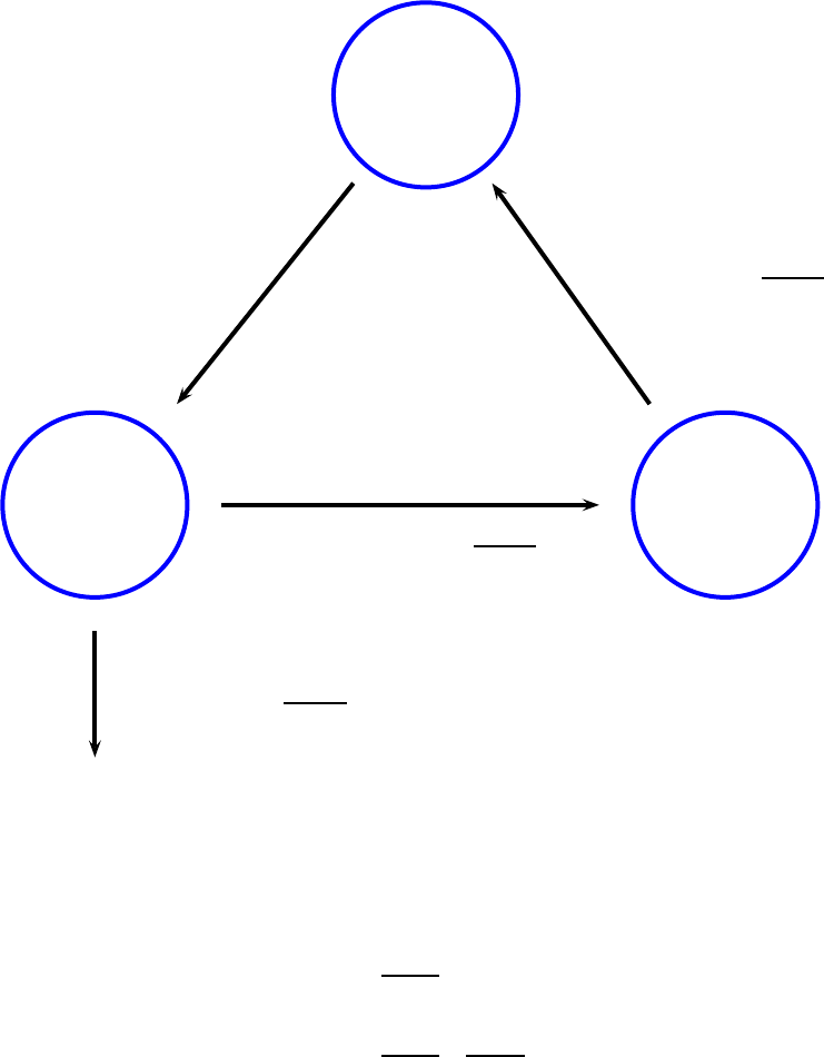
Figure 6: A Representation of the Relending Interpretation of the First-best

Warehouses

Farmers

invest i

1 + α

pay labor wℓ

αe

1 + α

Laborers

deposit d

αe

1 + α

lend L

= d

grain e

n+1

= L

we ﬁnd that

ℓ

∞

n=0

ℓ

(86)

∞

n=0

αe

1 + α

(87)

∞

n=0

1 + α



1 + α



e (88)

= αe. (89)

The ex press ions for i

and ℓ

under the relending model coincide with those in Proposi-

tion 3. Further, they suggest a natural money multiplier, stemming from the production

function. Of each unit of grain in the economy, a proportion 1/(1 + α) is invested in

capital and cannot be reused. The remainder is invested in labor, or working capital,

and therefore deposited back in the warehouse for reuse. These deposits are lend out,

and a proportion 1/(1 + α) is again invested in capital and the remainder is invested

in labor, which is deposited and reused. Thus, for every unit of grain, the amount that

can be invested is

∞

n=0



1 + α



= 1 + α. (90)

The multiplier Λ

corresponds to a money multiplier in classical banking models.

This is the liquidity multiplier of Section 6. Note that the more important working

capital (labor ℓ) is to production relative to physical capital (grain i), i.e. the higher is

α, the higher is the multiplier. Private money expands the money supply only to create

working capital. It cannot, of course, create physical capital out of thin air.

A.4 Table of Notations

Indices

f farmer index

l laborer index

b warehouse (bank) index

t ∈ {0, 1, 2} time index

Prices

deposit rate at Date t

lending rate at Date 0

w wages at Date 0

Demand and Supply

i grain farmers invest at Date 0

ℓ

labor farmers demand at Date 0

ℓ

labor laborers supply at Date 0

grain stored by player j at Date t

grain deposited in warehouses by farmers at Date t

grain deposited in warehouses by laborers at Date t

B loans demanded by farmers at Date 0

L loans supplied by warehouses at Date 0

overall deposits in warehouse at Date t

Production a nd Consumption

y farmer s’ output at Date 1

consumption o f player j at Date 2

Parameters

δ depreciatio n rate with private storag e

A productivity

α ratio of labor to grain in farmers’ production

e farmers’ (Date 0) endowment

E warehouses’ (Date 1) endowment (extension in Subsection 7.2)

γ cost parameter (extension in Subsection 7 .2)

Other Variables

farmer’s grain holding at Date 1

Λ liquidity multiplier

θ liquidity ratio (extension in Subsection 7.1)

∆ probability of spoilage (extension in Subsection 7.2)

central bank rate (extension in Subsection 7.3)

References

Allen, F., E. Carletti, and D. M. Gale (2014, September). Money, Financial Stability

and Eﬃciency. Journal of Economic Theory 149(8553), 100–127.

Allen, F. and D. Gale (1998). Optimal ﬁnancial crises. The Journal of Finance 53,

1245–1284.

Allen, F. and D. Gale (2004, July). Financial intermediaries and markets. Economet-

rica 72(4), 1023–1062.

Berger, A. N. and C. H. S. Bouwman (2009). Bank liquidity creation. The Review of

Financial Studies 22 (9), pp. 3779–3837.

Bolton, P. and D. S. Scharfstein (1990, March). A theory of predation based on agency

problems in ﬁnancial contracting. American Economic Review 80 (1), 93–106.

Brunnermeier, M. K. and L. H. Pedersen (2009). Market liquidity and funding liquidity.

Review of Financial Studies 22, 2201–2238.

Bryant, J. (1980). A model of reserves, bank runs, and deposit insurance. Journal of

Banking & Finance 4 (4), 335–344.

Calomiris, C. and D. Nissim (2014). Shifts in the market valuation of banking activities.

Journal of Financial Intermediation 23, 400–435.

Coval, J. D. and A. V. Thakor (2005). Financial intermediation as a beliefs-bridge

between optimists and pessimists. Journal of Financial Economics 75, 535–570.

Diamond, D. W. (1984). Financial intermediation and delegated monitoring. The

Review of Economic Studies 51 (3), pp. 393–414.

Diamond, D. W. and P. H . Dybvig (1983). Bank runs, deposit insurance, and liquidity.

Journal of Political Economy 91, 410–419.

Diamond, D. W. and R. G. Rajan (2001). Liquidity risk, liquidty creation, and ﬁnancial

fragility: A theory of banking. Journal of Political Economy 109, 287–327.

Freixas, X ., A. Martin, and D. Skeie (2011). Bank liquidity, interbank markets, and

monetary policy. Review of Financial S t udies 24 (8), 2656–2692.

Goodhart, C. A. (2010). The changing role of central banks. Working paper No. 326,

BIS.

Greenbaum, S., A. V. Thakor, and A. W. Boot (2015). Contemporary F inancial Inter-

mediation. Elsevier, Third Edition.

Hahn, A. (1920). Volkswirtschaftliche T heorie des Bankkredits. Tübingen: J.C.B. Mohr.

Hart, O. and J. Moore (1998, February). Default and renegotiation: A dynamic model

of debt. The Quarterly Journal of Economics 113 (1), 1–41.

Holmstrom, B. and J. Tirole (1997, August). Financial Intermediation, Loanable Funds,

and the Real Sector. The Quarterly Journal of Economics 112 (3), 663–91.

Holmström, B. and J. Tirole (2011). Inside and Outside Liquidity. The MIT Press.

Jacklin, C. (1987). Demand deposits, trading restrictions, and risk s haring. In

E. Prescott and N. Wallace (Eds.), C ontractual Arrangements for Intertemporal

Trade, Chapter II, pp. 26–47. Minneapolis: University of Minnesota Press.

Kashyap, A. K., R. Rajan, and J. C. Stein (2002, 02). Banks as Liquidity Providers:

An Explanation for the Coexistence of Lending and Deposit-Taking. Journal of

Finance 57 (1), 33–73.

Keeton, W. R. (1993). The impact of monetary policy on bank lending: The role of

securities and large CDS. Econ omic Review, The Federal Reserve Bank of Kansas

City, 35–47.

Knapp, G. F. (1924). The State Theory of Money. Number knapp1924 in History of

Economic Thought Books. McMaster University Archive for the History of Economic

Thought.

Lawson, W. (1855). The History of Banking. London: Richard Bentley.

Macmillan Committee (1931). British Parliamentary Reports on Interantional Finance:

The Report of the Macmillan Committee. London: H.M. Stationery Oﬃce.

Minsky, H. (2008). Stabilizing an Unstable Economy. McGraw-Hill.

Mishkin, F. (2010). Monetary policy strategy: Lessons from the crisis. Working paper,

Columbia University.

Pennacchi, G. (2012). Narrow banking. Annual Review of Fi nancial Economics 4,

141–159.

Postlewaite, A. and X. Vives (1987, June). Bank Runs as an Equilibrium Phenomenon.

Journal of Political Economy 95(3), 485–91.

Ramakrishnan, R. T. S. and A. Thakor (1984). Information reliability and a theory of

ﬁnancial intermediation. Review of Economic Studies 51 (3), 415–32.

Skrastins, J. (2015). Firm boundaries and ﬁnancial contracts . Working paper.

Werner, R. A. (2014). Can banks individually create money out of nothing? theories

and empirical evidence. Review of Financial Analysis 36, 1–19.

Wicks ell, K. (1907). The inﬂuence of the rate of interest on prices. Econ om ic Journal 17,

213–220.

Williams, J. (1986). Fractional reserve banking in grain. Journal of Money, Credit and

Banking 16, 488–496.